PolyCalAPP
PolylCalAPP is a MATLAB application for comparative polynomial calibration based on the algorithm PolylCa. PolylCalAPP is part of CharFunTool.
PolylCalAPP allows to specify the uncertainty budget of the direct measurements in the calibration experiment and estimates the patrameters of the polynomial calibration function together with their uncertainties.
Contents
Details
PolyCal is an alternative approach for estimating the calibration parameters together with their associated uncertainties and, moreover, with their derived state-of-knowledge distributions, based on the EIV (Errors-In-Variables) modeling approach [4] and the characteristic function approach [5-6]. For detailed description of the suggested concept for polynomial comparative calibration see [7-8].
In metrology, the straight-line calibration and the polynomial calibration problem is addressed in the ISO Technical Specifications ISO/TS 28037:2010 and ISO/TS 28038:2018 which are based on the GUM uncertainty framework defined in GUM[3] using the law of propagation of uncertainty.
Here, in the considered calibration experiment, the direct measurements taken by two independent measurement devices are represented by  -dimensional vectors
\begin{align}\label{eq1} \mathbf X &= \boldsymbol \mu + E_{\mathcal X} = \boldsymbol \mu + \left(\mathbf X^{A} + \mathbf X^{B} + X^{B}_0 \mathbf 1 \right),\\ \mathbf Y &= \boldsymbol \nu + E_{\mathcal Y} = \boldsymbol \nu + \left(\mathbf Y^{A} + \mathbf Y^{B} + Y^{B}_0 \mathbf 1 \right), \label{eq1b} \end{align}
\[ E \begin{pmatrix} \mathbf X\\ \mathbf Y \end{pmatrix} = \begin{pmatrix} \boldsymbol \mu\\ \boldsymbol \nu \end{pmatrix}, \quad \mathop{\mathrm{Cov}} \begin{pmatrix} \mathbf X\\ \mathbf Y \end{pmatrix} = \mathbf \Sigma = \begin{pmatrix} \mathbf \Sigma_{\mathcal X} & \mathbf \Sigma_{\mathcal X,\mathcal Y}\\ \mathbf \Sigma_{\mathcal Y,\mathcal X} & \mathbf \Sigma_{\mathcal Y} \end{pmatrix} \]
where \(\boldsymbol \mu = \left(\mu_1,\dots,\mu_m\right)'\) and \( \boldsymbol \nu = \left(\nu_1,\dots,\nu_m\right)'\) represent the true unknown values of the measurands expressed in units of the measuring devices. These parameters are functionally related by the polynomial calibration function,
\[ \boldsymbol \nu = \beta_0 \boldsymbol 1 + \beta_1 \boldsymbol \mu + \beta_2 \boldsymbol \mu^2 + \cdots + \beta_p \boldsymbol \mu^p \]
The components of the measurement errors are assumed to be mutually independent zero-mean random variables, fully specified by their probability distributions (here by their characteristic functions)derived by Type A and Type B methods of evaluation.
PolyCal estimates the patrameters of the polynomial calibration function \(\boldsymbol \beta = (\beta_0,\dots,\beta_p)'\) together with their uncertainties (covariance matrix) and their marginal state-of-knowledge distributions. Moreover, the algorithm evaluates the fitted values \(y_{Fit}\) of the calibration function for given \(x_{Fit}\),
\[ y_{Fit} = \beta_0 + \beta_1 x_{Fit}^{} + \beta_2 x_{Fit}^2 +\cdots + \beta_p x_{Fit}^p, \]
together with their uncertainties and the state-of-knowledge distributions. The output from the PolyCal algorithm can be further used to evaluate the results of the future measurements by the calibrated instrument, together with their uncertainties and the state-of-knowledge distributions.
SYNTAX
result = PolyCal(x,y,xFit,options)
result = PolyCal(x,y)
result = PolyCal(x,y,[],options)
EXAMPLE
Comparative polynomial calibration with artificial data
MATLAB Code
x = [4.7, 5.5, 6.5, 7.5, 8.4]';
y = [5.8, 7.9, 10.4, 12.7, 15.2]';
xFit = linspace(5,8,11)';
clear options
options.order = 1;
options.cfXA = {@(t)cf_Normal(0.01*t), ...
    @(t)cf_Normal(0.1*t), ...
    @(t)cf_Normal(0.1*t), ...
    @(t)cf_Student(0.1*t,5), ...
    @(t)cf_RectangularSymmetric(0.2*t)};
options.cfXB = {@(t)cf_RectangularSymmetric(0.1*t), ...
    @(t)cf_RectangularSymmetric(0.1*t), ...
    @(t)cf_TriangularSymmetric(0.1*t), ...
    @(t)cf_TriangularSymmetric(0.1*t), ...
    @(t)cf_RectangularSymmetric(0.2*t)};
options.cfXB0 = [];
options.cfYA = {@(t)cf_Normal(0.15*t), ...
    @(t)cf_Normal(0.2*t), ...
    @(t)cf_Normal(0.2*t), ...
    @(t)cf_Normal(0.3*t), ...
    @(t)cf_Normal(0.3*t)};
options.cfYB = {@(t)cf_RectangularSymmetric(0.2*t), ...
    @(t)cf_RectangularSymmetric(0.2*t), ...
    @(t)cf_TriangularSymmetric(0.3*t), ...
    @(t)cf_TriangularSymmetric(0.3*t), ...
    @(t)cf_RectangularSymmetric(0.3*t)};
options.cfYB0 = @(t)cf_ArcsineSymmetric(0.1*t);
options.tolDiff = 1e-2;
result = PolyCal(x,y,xFit,options);
%
%
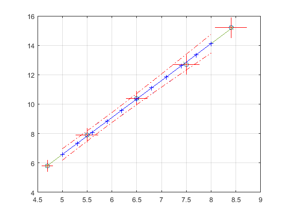
EXAMPLE - continued
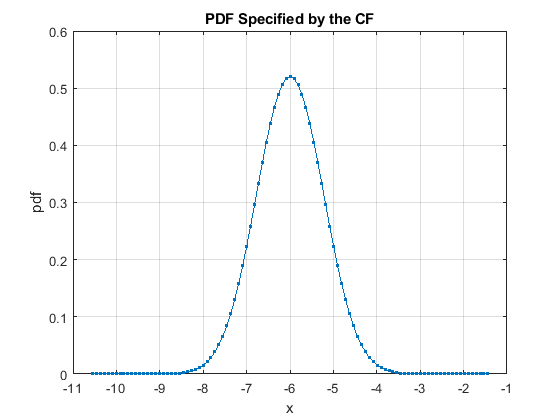
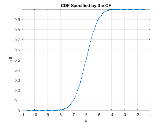
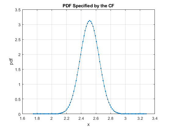
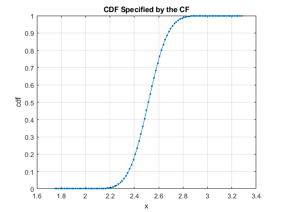
Plot the PDF/CDF of the parameters
MATLAB Code
cfBeta = result.cfBeta;
resultBeta0 = cf2DistGP(cfBeta{1},[],[],options);
figure;
resultBeta1 = cf2DistGP(cfBeta{2},[],[],options);

%
REFERENCES
- ISO/TS 28037:2010. Determination and Use of Straight-Line Calibration Functions. International StandardsOrganization, Geneva, September (2010).
- ISO/TS 28038:2018. Determination and Use of Polynomial Calibration Functions. International Standards Organization, Geneva, December (2018).
- JCGM 100:2008. Evaluation of measurement data – Guide to the expression of uncertainty in measurement (GUM 1995 with minor corrections), ISO, BIPM, IEC, IFCC, ILAC, IUPAC, IUPAP and OIML, (2008).
- KUBÁČEK L. Foundations of Estimation Theory, Elsevier, Amsterdam (1988).
- WITKOVSKÝ V. Numerical inversion of a characteristic function: An alternative tool to form the probability distribution of output quantity in linear measurement models. ACTA IMEKO 5 (3), (2016) 32–44.
- WITKOVSKÝ V. CharFunTool: The Characteristic Functions Toolbox (MATLAB). https://github.com/witkovsky/CharFunTool, (2020).
- WITKOVSKÝ V. and WIMMER G. Generalized polynomial comparative calibration: Parameter estimation and applications. In: Advances in Measurements and Instrumentation: Reviews. S.Y. Yurish (Ed.). Barcelona, Spain, IFSA (International Frequency Sensor Association Publishing) Publishing S.L., (2018) 15-52.
- WITKOVSKÝ V. and WIMMER G. PolyCal - MATLAB algorithm for comparative polynomial calibration and its applications. AMCTM 2020.